Heritability (3): Non-additive effects dominance

Dominance is a just a fancy-schmancy way of saying that the phenotypic effects of alleles at a single locus are not additive 💁‍♂️. Ok, but what does that mean?

To illustrate, let’s go back to the example of differences in milk-yield among a bunch of cows 🐮🐮(Fig. 1). As I mentioned in a previous post, some of these differences are due to genetic differences among the cows and some are due to environmental differences. For example, there could be (average) differences between the milk yield of cows with AA genotype (30 liters) vs cows with Aa genotype (20 liters) vs cows with aa genotype (10 liters). In this example, each additional A allele results in an (average) increase of 10 liters of milk (Fig. 1A). This may not always be the case if, for example, cows with the Aa genotype and AA genotype have the same average milk yield: 30 liters (Fig 1B). If this is the case, we say that the effect of alleles at this locus are non-additive or that there is dominance at this locus.

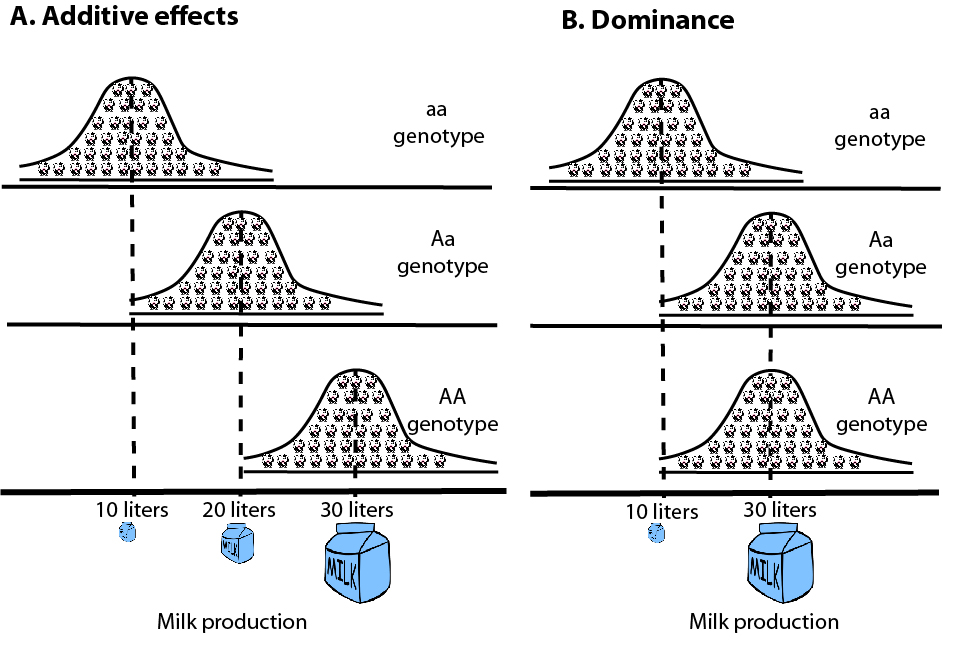Fig. 1: A) Additivity is when each additional allele adds a fixed value to the phenotype. B) Things are not that symmetric when there’s dominance. In this example, the average phenotype is the same for the AA and Aa genotypes.

When you were learning genetics in school 🏫, you probably came across terms like “dominant” and “recessive”, which are often used to refer to Mendelian traits such as the presence/absence of cleft chin 🍑 in humans. These terms are ok for simple Mendelian traits but quite limiting for quantitative traits . Also limiting are terms like complete dominance, a special case of dominance in which the phenotypic distributions of AA and Aa genotypes are indistinguishable (Fig. 1B). There is a more flexible way to describe dominance: d.

The dominance deviation, d, describes the degree (and direction) in which genotypic values deviate from additivity.

🛑✋ Sidebar: It’s useful to define genotypic value here as it is an important concept in quantitative genetics. The genotypic value is the average phenotype of a specific genotype. For example, the genotypic value of the Aa genotype in Fig. 1A is 20 liters. So even though some individuals carrying the Aa genotype have higher or lower milk yields because of environmental differences among them, they all yield, on average, 20 liters of milk. Thus, the genotypic value is supposed to represent the ‘true’ phenotypic effect of the genotype. It is often convenient to represent genotypic values as deviations from the mean of the population. For example, the genotypic value of the aa genotype in Fig. 1A can be written as 10 - 20 = -10 (instead of 10) if we assume the average milk yield in the population is 20 liters. This is mostly for convenience sake in calculations so don’t worry too much about this. Sidebar over.👍

Now take a look at Fig. 2 and give it some time.🤔

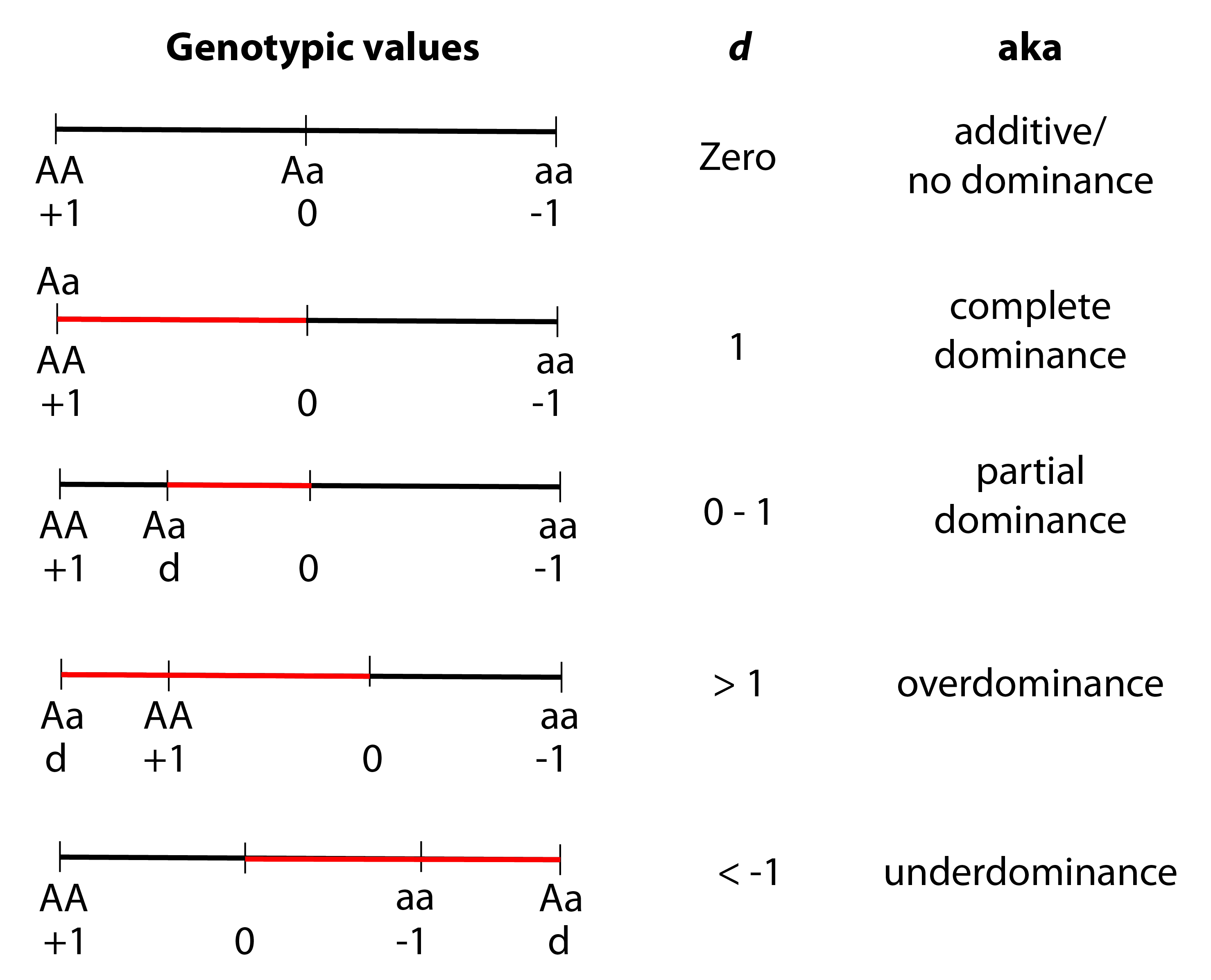Fig. 2: Different values of d describe different cases of dominance. The scale represents the genotypic values, where +1 and -1 refer to the genotypic values of AA and aa, respectively, expressed as scaled deviations from the mean. The red line, which represents the scaled dominance deviation, shows the extent to which the genotypic value of the heterozygote Aa deviates from what we expect had the allelic effects been completely additive.

Can you see how the dominance deviation flexibly and quantitatively describes the different cases of dominance (including no dominance!)? The meaning of the different values of d are further explained below:

d = 0: no dominance. The allelic effects are completely additive and the average phenotype of Aa is smack dab in the middle between AA and aa.

d = 1: complete dominance. AA has the same genotypic value as Aa. Note that this is the same as the example of milk yield in Fig. 1B.

0 > d > 1: partial dominance. The genotypic value of Aa lies somewhere between that of AA and aa. As d gets closer to 1, the genotypic value of Aa gets closer to that of AA.

d > 1: overdominance. This is when the genotypic value of Aa is greater than that of either homozygote. So, for example, the average milk yield of cows carrying the Aa genotype might greater than the average milk yield of cows carrying the AA or aa genotype. This is sometimes referred to as hybrid vigor.

d < -1: underdominance. The genotypic value of Aa is less than that of either homozygote.

🚨There is one common misconception regarding dominance that I want to clear up: dominance does not tell us anything about how frequent the allele is in the population. For example, the A allele in Fig. 1B, even though it is ‘dominant’, might only be present at 10% frequency in the population.

Dominance is only one example of non-additive effects of alleles on the phenotype. So far I have only talked about the phenotypic effects of alleles at a single locus. What happens if we consider alleles at two or more loci? We’re faced with non-additive effects of alleles across loci. Non-additive effects of alleles at two or more loci are called epistasis and I plan to talk about this next time. See you in a couple of months…📆