Why we expect genetic differences between populations to be zero

The expected genetic value in a population

To answer these questions, we must first talk about genetic value and figure out what it’s expectation is in a single (randomly mating) population. Let’s begin (as we do) with a generative model for the phenotype:

\[y = g + e\]

where \(g = \sum_{i = 1}^M \beta_i x_i\) is the genetic value (summed across \(M\) loci) and \(e\) is random (environmental) error. I like to think of the genetic value as the expected phenotype of an individual given their genotype (\(x\)): \(\mathbb{E}(y|x)\). You can also (informally) think of it as the phenotype of an individual that can be predicted from their genotype.

Assuming only additive effects, we can write the genetic value of each genotype at the \(i^{th}\) (biallelic) locus (\(x_i \in \{0,1,2\}\)) as \(\mathbb{E}(y|x_i = 0) = 0\), \(\mathbb{E}(y|x_i = 1) = \beta_i\), and \(\mathbb{E}(y|x_i = 2) = 2\beta_i\) ¹. From this, we can get the mean genetic value in the population by marginalization. Let’s denote the frequency of the \(i^{th}\) variant in the population as \(f_i\). Then,

\[\begin{aligned} \mathbb{E}(y) = & \mathbb{E}\{\mathbb{E}(y|x_i)\} \\ = & \mathbb{E}(y|x_i = 0)\mathbb{P}(x_i = 0) + \mathbb{E}(y|x_i = 1)\mathbb{P}(x_i = 1) + \\ & \mathbb{E}(y|x_i = 2)\mathbb{P}(x_i = 2) \\ = & 0(1 - f_i)^2 + \beta_i\{2 f_i (1 - f_i)\} + 2\beta_i(f_{i}^2) \\ = & 2\beta_i f_i - 2\beta_i f_i^2 + 2\beta_i f_i ^2 \\ = & 2\beta_i f_i \end{aligned}\]

Where \(\mathbb{P}(x_i = 0)\) is the frequency of individuals carrying 0 copies of the (effect) allele in a randomly mating population, \(\mathbb{P}(x_i = 1)\) is the frequency of individuals carrying 1 copy and so on. Aggregating this across multiple independent (unlinked) causal loci gives us the mean genetic value in a single population: \(\mathbb{E}(y) = 2\sum_{i=1}^M\beta_i f_i\). To demonstrate this, note that \(\mathbb{E}(y|x_i) = \beta_ix_i\) and \(\mathbb{E}(y|x) = \sum_i^M \beta_ix_i\). Therefore,

\[\begin{aligned} \mathbb{E}(y) = & \mathbb{E}\{\mathbb{E}(y|x)\} \\ = & \mathbb{E}\left( \sum_{i= 1}^M \beta_i x_i \right) = \sum_{i = 1}^M \beta_i \mathbb{E}\left( x_i \right) \\ = & \sum_{i = 1}^M \beta_i 2 f_i = 2 \sum_{i = 1}^M \beta_i f_i \end{aligned}\]

From this it follows that the mean genetic value in populations 1 and 2 are \(\mathbb{E}(g_1) = 2\sum_{i = 1}^M\beta_i f_{i}^{(1)}\) and \(\mathbb{E}(g_2) = 2\sum_{i = 1}^M\beta_i f_{i}^{(2)}\), respectively, where \(f_{i}^{(1)}\) and \(f_{i}^{(2)}\) are the allele frequencies in populations 1 and 2, respectively. Note, that I’m assuming that the causal effect size is the same across populations. The expected difference in genetic values between the two populations is then \(2\sum_{i=1}^M\beta_if_{i}^{(1)} - 2\sum_{i = 1}^M\beta_if_{i}^{(2)} = 2\sum_{i = 1}^M\beta_i(f_{i}^{(1)} - f_{i}^{(2)})\). In this expression, \(\beta_{i}\)s are fixed and \(f_{i}^{(1)} - f_{i}^{(2)}\) are random (over the evolutionary process), which means that to understand the expected mean difference in genetic value between populations, we need to work out the expected difference in allele frequency.

Expected difference in allele frequency between populations

For two (randomly mating) populations that have diverged from a common ancestral population ², the frequency of a neutral allele in the \(j^{th}\) population at the \(i^{th}\) locus approximately follows a normal distribution:

\[f_{i}^{(j)} \sim \mathcal{N}(f_i ~, ~ f_i(1-f_i)F)\] Where \(f_i\) is the frequency in the ancestral population and \(F\) is a measure of drift since the populations split. \(F \approx \frac{t}{2N_e}\) where \(t\) is the number of generations since the split and \(N_e\) is the (diploid) effective population size. You can also think of \(F\) as the \(F_{st}\) between the two populations (more on this some other time). The derivation for this is complicated and not super important for this post but I’ll demonstrate that it holds with simulations.

library(dplyr)
library(ggplot2)
library(data.table)

Write a function to simulate drift in a population given some starting frequency, the effective population size, and the number of generations for which we want the simulation to run.

#write a binomial sampling function to simulate drift in a population
let.it.drift <-function(f0, g, Ne){
  #f0 is  starting frequency in the ancestral population
  #make sure g and Ne are integers
  for(i in 1:g){
    nalleles = rbinom(Ne, 2, f0) #sample Ne diploid individuals
    f0 = mean(nalleles)/2 #calculate frequency in the population
  }
  return(f0) # return final frequency
}

Now simulate the drift in the allele frequency at 1,000 independent loci, each starting with an ancestral frequency of 0.5. We’ll simulate a population of size 1,000 individuals and see how the frequency changes as we increase the divergence time between the two populations.

#simulate drift in 1000 loci for increasing number of generations of drift (5-50)
p.exp = sapply(seq(5,50,10),
               function(x){
                 replicate(1000, let.it.drift( f0 = 0.5, g = x, Ne = 1000))})

p.exp = data.table(p.exp)
colnames(p.exp) = as.character(seq(5,50,10))
p.exp$rep = c(1:1000)

# melt to long format for plotting in panels
mp.exp = reshape2::melt(p.exp, id.vars="rep", 
              variable.name = "generations",
              value.name = "frequency")

#calculate the expected and observed mean and variance in allele frequency for each value of the number of generations
mp.exp.summary = mp.exp %>%
  group_by(generations)%>%
  summarize(mean.f = mean(frequency),
            var.f = var(frequency)) %>%
  mutate(g = as.numeric(as.character(generations)),
         exp.var = 0.5*(1 - 0.5)*(g/2000))

## `summarise()` ungrouping output (override with `.groups` argument)

#plot!
ggplot(mp.exp, aes(frequency))+
  geom_histogram()+
  facet_grid(generations~.)+
  theme_classic()+
  geom_vline(xintercept = 0.5, 
             color = "Red", 
             linetype= "dashed")+
  geom_vline(data = mp.exp.summary, 
             aes(xintercept = mean.f), 
             color = "blue",
             linetype= "dashed")+
  geom_text(data = mp.exp.summary, 
            aes(x = 0.65, y = 100, 
                label = paste("obs. var", 
                              round(var.f,4))),
            color = "blue")+
  geom_text(data = mp.exp.summary, 
            aes(x = 0.65, y = 200, 
                label = paste("exp. var",
                              round(exp.var,4))),
            color = "red")+
  labs(x = "Frequency",
       y = "Count")

## `stat_bin()` using `bins = 30`. Pick better value with `binwidth`.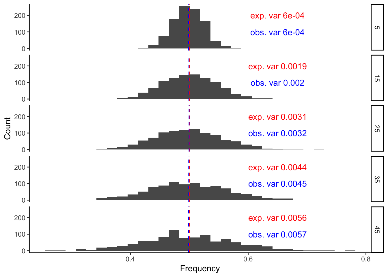

Notice a few things:

1. The observed mean (red line) and variance (red text) in allele frequency closely match those predicted from the model above, even for populations (of 1,000 individuals) that diverged 45 generations ago.

2. Even though the allele frequency at any single locus can vary substantially from the ancestral frequency, the mean of the distribution (representing the expected allele frequency) does not change regardless of how many generations of drift we simulate.

3. However, what does increase as a function of the number of generations is the variance (or spread) of the allele frequency distribution. In other words, even though we expect the allele frequency to remain the same (regardless of the number of generations), the possible values that the frequency can reach (in either direction) gets larger and larger with every generation.

Because the expected frequency in both populations is the same, i.e., \(\mathbb{E}(f_i^{(1)}) = \mathbb{E}(f_i^{(2)}) = f_i\), the expected difference in allele frequency between the two populations \(\mathbb{E}(f_i^{(1)} - f_i^{(2)}) = \mathbb{E}(f_i^{(1)}) - \mathbb{E}(f_i^{(2)}) = 0\). And the expected mean difference in genetic value is \(\mathbb{E}(g_1 - g_2) = 2\sum_{i = 1}^M\beta_i\mathbb{E}(f_{i}^{(1)} - f_{i}^{(2)}) = 0\).

In other words, we expect the genetic difference underlying a phenotype between populations to be zero. Does that mean that we don’t expect to see any differences between populations? No, because even though the expected difference in frequency is zero, the expected absolute difference is not zero. Let me illustrate this by simulating drift in two populations that have evolved independently since their divergence from a common ancestral population with allele frequency of 0.5.

#simulate drift in 1000 loci for increasing number of generations of drift (5-50)
#pop 2 (we will use p.exp as pop1 frequencies)
p.exp2 = sapply(seq(5,50,10),
               function(x){
                 replicate(1000, let.it.drift( f0 = 0.5, g = x, Ne = 1000))})

p.exp2 = data.table(p.exp2)
colnames(p.exp2) = as.character(seq(5,50,10))
p.exp2$rep = c(1:1000)

# melt to long format for plotting in panels
mp.exp2 = reshape2::melt(p.exp2, id.vars = "rep", 
              variable.name = "generations",
              value.name = "frequency")

colnames(mp.exp)[3] = "freq1"
colnames(mp.exp2)[3] = "freq2"

mp.exp = merge(mp.exp, mp.exp2, by = c("rep","generations"))

#calculate the expected and observed mean and variance in allele frequency for each value of the number of generations
mp.exp.summary = mp.exp %>%
  group_by(generations)%>%
  summarize(mean.abs.diff = mean(abs(freq1 - freq2)))

## `summarise()` ungrouping output (override with `.groups` argument)

#plot!
ggplot(mp.exp, aes(abs(freq1 - freq2)))+
  geom_histogram()+
  facet_grid(generations~.)+
  theme_classic()+
  geom_vline(data = mp.exp.summary, 
             aes(xintercept = mean.abs.diff), 
             color = "blue",
             linetype= "dashed")+
  labs(x = bquote("Absolute difference in allele frequency : abs("~f^(1)~"-"~f^(2)~")"),
       y = "Count")

## `stat_bin()` using `bins = 30`. Pick better value with `binwidth`.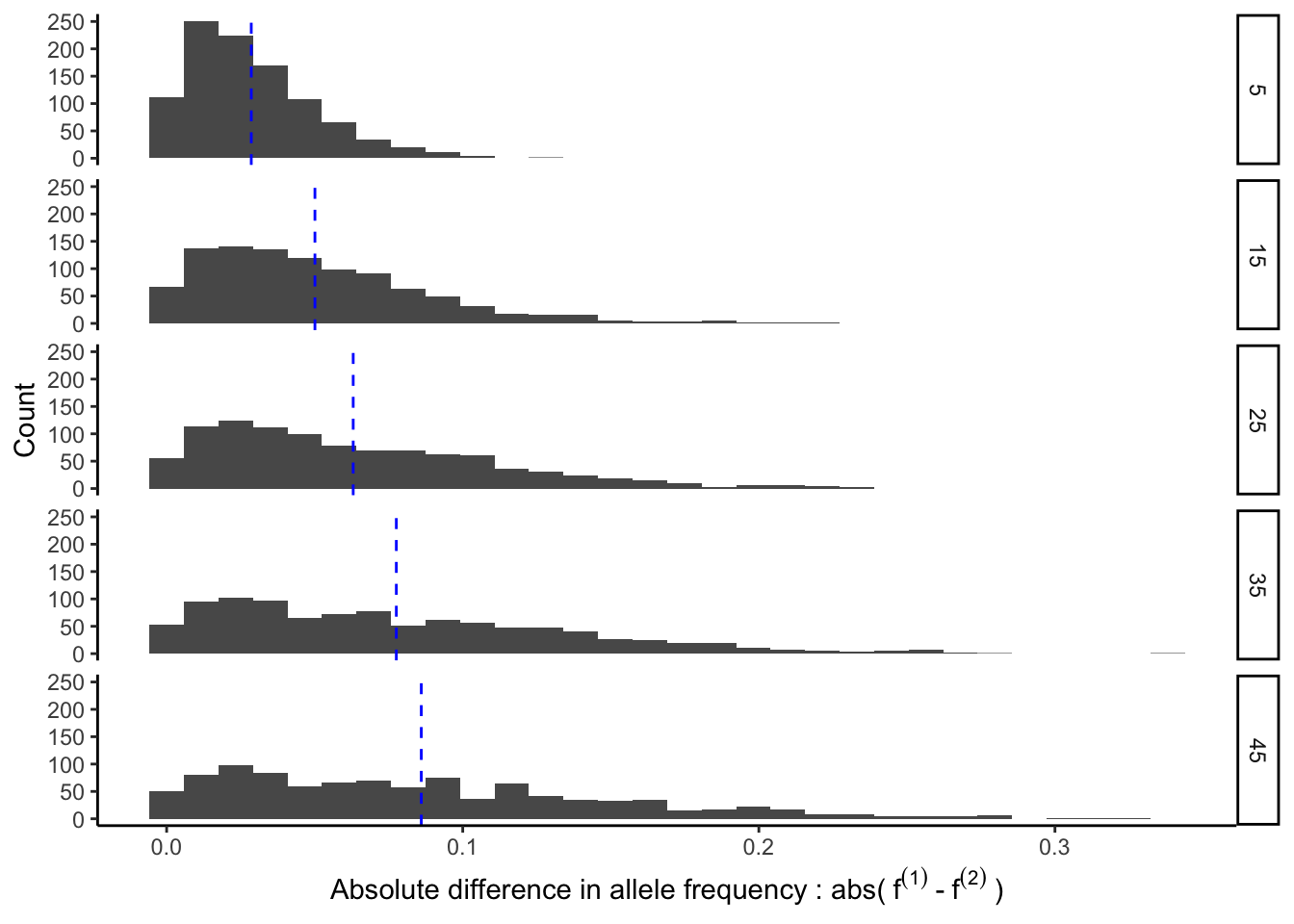

The figure above shows that the expected absolute difference in allele frequency between the two populations is not zero. In fact, it increases as a function of divergence time (blue line in the plot above). In other words, the more diverged the populations, the more we can expect there to be allele frequency differences between them.

It follows then that we also expect the absolute difference in genetic values between populations to also increase with divergence time.

A simpler way to say this is that for two populations that diverged from some common ancestor, we do expect there to be genetic differences underlying a neutrally evolving trait. BUT, we don’t know which direction this difference will take. Putting it differently, we don’t know whether population 1 or 2 should have a higher mean genetic value for the trait. This is one thing that needs to be kept in mind when discussing phenotypic differences between populations.

Can we not infer this from the direction of the phenotypic difference? Say if population 1 has a higher phenotypic value than populaion 2, can we say anything about the direction of underlying genetic difference? No. so far I’ve only discussed the variation in the genetic component (\(g\) in our phenotype model). The direction of phenotypic difference is also driven by the environment, which could be different between the two populations. More on this some other time but in conclusion:

1. The expectation of the genetic difference underlying a trait between populations is zero.

2. But this does not mean that there won’t be any genetic difference between populations. In fact, we expect this difference to increase with divergence time.

3. However, we cannot predict (for a neutral trait) which direction the difference is going to take, i.e, we cannot say if population 1 or 2 will have a higher genetic value.

I should point that these conclusions are only applicable to neutral traits. Under directional selection, we do expect systematic differences in mean genotypic value between populations. However, as mentioned earlier, this cannot be inferred directly from differences in phenotypic means between populations. And even differences in genetic means between populations may not be due to selection. More on this at some other undecided time in the future…