A general model for the bias in variant effect sizes due to population structure

Motivation

The effects of population structure in GWAS (genome-wide association studies) have been well-studied. It’s one of those problems that on a surface level is quite easy to grasp intuitively. And that sort of understanding is fine for most practical purposes. However, there’s still a lot of confusion around how population structure impacts/biases variant effect sizes, even among geneticists and particularly with respect to the difference between genetic and environmental stratification. I think some of this stems from a lack of good/easy/clear statistical descriptions of the effect of population stratification on GWAS. I worked this out while working on a recent paper ¹ so I decided to post it in case others find it helpful.

The phenotype model

We begin by stating a generative model for some heritable phenotype $y$:

$$\begin{array}{r}y=\mu +g+s+e\end{array}$$

Here, $\mu$ is the mean phenotypic value in the population, $g$ is the genotypic value (or true polygenic score), $s$ is some environmental effect (I’m only assuming one here), and $e$ is random error. Furthermore, $g=\sum _{i=1}^m{\beta }_i{x}_i$, where $x_i$ is the genotype and ${\beta }_i$ is the (true) effect size of the $i^{th}$ (out of $m$) causal variants.

The estimated effect size of a variant

The ordinary least squares (OLS) effect size estimate of a predictor $X$ on some response $Y$ is $\frac{cov(Y,X)}{var(X)}$. Thus, in a GWAS with population structure, the effect estimate of the $j^{th}$ (test) variant is:

$$\begin{array}{rl}\widehat{{\beta }_j}& =\frac{cov(y,x_j)}{var(x_j)}\\ & =\frac{cov(\mu +g+s+e,x_j)}{var(x_j)}\\ & =\frac{cov(\mu ,x_j)+cov(g,x_j)+cov(s,x_j)+cov(e,x_j)}{var(x_j)}\end{array}$$

In expectation, $cov(\mu ,x_j)=0$ because $\mu$ is a constant, and $cov(e,x_j)=0$ because $e$ is random with respect to $x_j$. Thus,

$$\begin{array}{rl}\mathbb{E}(\widehat{{\beta }_j})& =\frac{cov(g,x_j)+cov(s,x_j)}{var(x_j)}\end{array}$$

Now, we know that $g=\sum _{i=1}^m{\beta }_i{x}_i$. Thus, we can write $cov(g,x_j)$ as:

$$\begin{array}{rl}cov(g,x_j)& =cov(\sum _{i=1}^m{\beta }_i{x}_i,x_j)\\ & =cov({\beta }_1{x}_1,x_j)+cov({\beta }_2{x}_2,x_j)+\cdot \cdot \cdot \\ & +cov({\beta }_j{x}_j,x_j)+\cdot \cdot \cdot +cov({\beta }_m{x}_m,x_j)\\ & ={\beta }_{1}cov(x_1,x_j)+{\beta }_{2}cov(x_2,x_j)+\cdot \cdot \cdot \\ & +{\beta }_{j}cov(x_j,x_j)+\cdot \cdot \cdot +{\beta }_{m}cov(x_m,x_j)\\ & ={\beta }_{j}var(x_j)+\sum _{i=1,i\ne j}^m{\beta }_{i}cov(x_i,x_j)\end{array}$$

And the expected estimated effect size becomes:

$$\begin{array}{rl}\mathbb{E}(\widehat{{\beta }_j})& =\frac{cov(g,x_j)+cov(s,x_j)}{var(x_j)}\\ & =\frac{{\beta }_{j}var(x_j)+\sum _{i=1,i\ne j}^m{\beta }_{i}cov(x_i,x_j)+cov(s,x_j)}{var(x_j)}\\ & ={\beta }_j+\frac{\sum _{i=1,i\ne j}^m{\beta }_{i}cov(x_i,x_j)}{var(x_j)}+\frac{cov(s,x_j)}{var(x_j)}\end{array}$$

Thus, the expected effect size estimate of a variant in a GWAS with population structure can be written as a sum of its own true effect size ${\beta }_j$ and two sources of bias:

1. $\frac{\sum _{i=1,i\ne j}^m{\beta }_{i}cov(x_i,x_j)}{var(x_j)}$, from background genetic effects (aka genetic stratification).

2. $\frac{cov(s,x_j)}{var(x_j)}$ from confounding environmental effects (aka environmental stratification).

Genetic stratification

Population structure induces long-range LD (linkage disequilibirum) between variants across the genome. This causes the estimated effect size of the test variant $j$ to be influenced by the effect of all other causal variants (weighted by their LD with the test variant). This effect is often referred to as background genetic effect or genetic stratification. The total bias due to this effect is: $\frac{\sum _{i=1,i\ne j}^m{\beta }_{i}cov(x_i,x_j)}{var(x_j)}$.

In a panmictic population, $cov(x_i,x_j)$ will be very small or zero in expectation as long as the $i^{th}$ and $j^{th}$ variants are not physically close to each other. As the population becomes more and more structured, the overall LD between the test variant and all other causal variants, and therefore, the bias due to background genetic effects increases. Note, however, that if the effect size of the test variant is small (a realistic assumption), then, we can simply write this (background) term as:

$$\begin{array}{rl}& \frac{\sum _{i=1,i\ne j}^m{\beta }_{i}cov(x_i,x_j)}{var(x_j)}\\ \approx & \frac{\sum _{i=1}^m{\beta }_{i}cov(x_i,x_j)}{var(x_j)}\\ \approx & \frac{cov(g,x_j)}{var(x_j)}\end{array}$$

In other words, the bias due to background genetic effects can also be thought of as coming from the correlation between the test variant and the genotypic values (or true polygenic scores) in the population.

Environmental stratification

Any (known and unknown) environmental factor ($s$) that (a) affects the phenotype and (b) is correlated with the test variant (i.e. if $cov(s,x_j)\ne 0$), will also add to the bias in its effect size estimate. This bias can either be positive or negative depending on the sign of $cov(s,x_j)$.

To illustrate, imagine a phenotype (let’s say height) which is influenced by the latitude at which individuals live such that people in the north tend to be taller and people in the south tend to be shorter (for whatever reason). Let’s denote the latitude of the $k^{th}$ individual as $z_k$ and the effect size of latitude on the phenotype as $\gamma$ such that $s_k=\gamma z_k$. Then, $cov(s,x_j)=cov(\gamma z,x_j)=\gamma cov(z,x_j)$. Thus, the contribution of environmental stratification depends on (a) the correlation between the variant frequency and the environmental effect (i.e. $cov(z,x_j)$, which varies across variants), and (b) the effect size of the environment $\gamma$, which affects all variants equally.

This is demonstrated in the figure below, which shows the true effect size on the x-axis and estimated effect size on the y-axis with colors representing the direction and magnitude of the correlation between frequency and latitude.

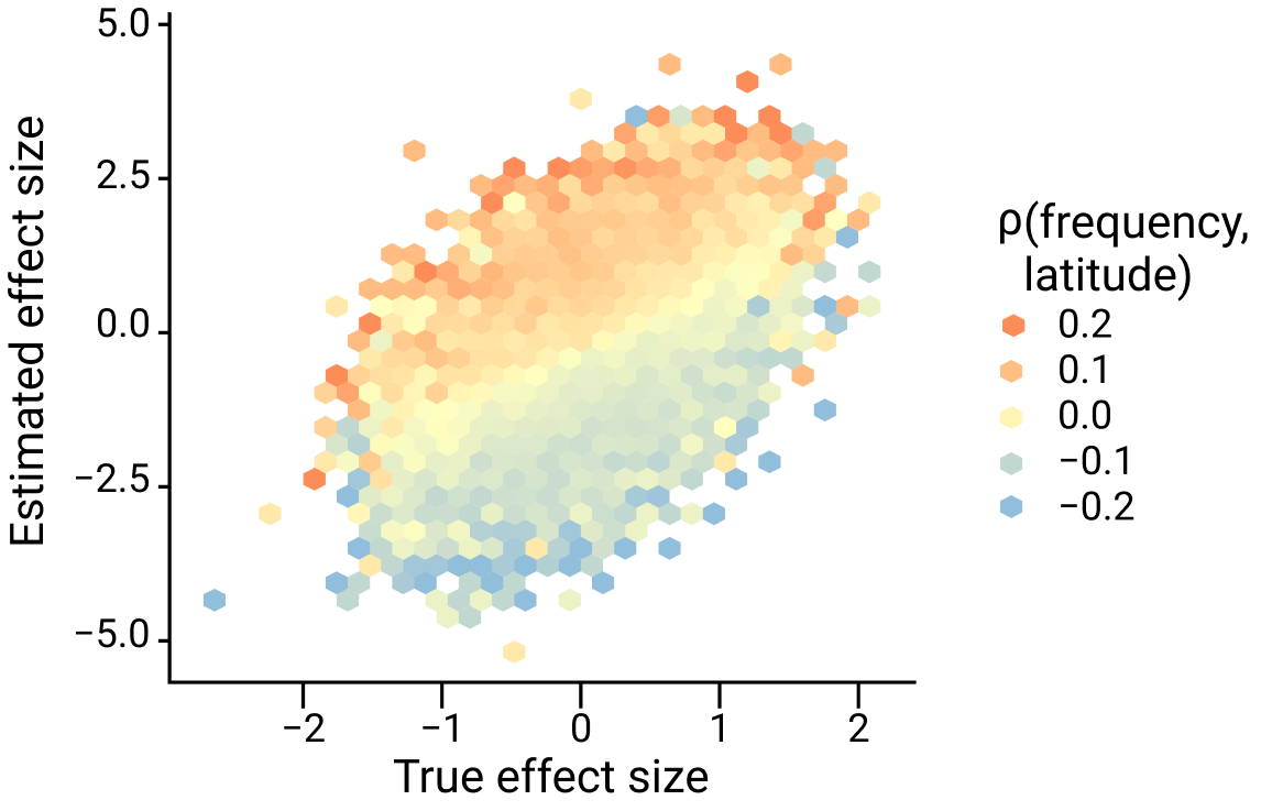
Figure adapted from Zaidi and Mathieson eLife 2020

Notice a few things:

1. The effect size of any variant whose frequency is correlated with latitude (i.e. for which $cov(z,x_j)\ne 0$) tends to deviate away from the diagonal (the true effect size).

2. The effect size of alleles that are positively correlated with latitude (red colors) tends to be inflated (lies above the diagonal) whereas alleles that are negatively correlated with latitude (blue colors) tend to be biased downwards (below the diagonal).

3. The degree of this bias is greater for variants that are more strongly correlated with latitude (darker colors).

In summary, the estimated effect size of the $j^{th}$ variant can be upwards or downwards, depending on the direction and magnitude of $cov(s,x_j)=\gamma cov(z,x_j)$.

Technically, the allele frequency of a given variant could be correlated with an environmental effect (and therefore bias its effect size) even in unstructured/randomly mating populations (just by chance). But, this is very unlikely in an unstructured population. With more structure in the population, the distribution of allele frequencies in the population becomes less random, increasing the probability that they will be correlated with environmental effects. The LD between causal variants will increase as well (multi-locus Wahlund effect). Altogether, population structure will introduce bias in the effect size through both background genetic effects and environmental stratification.