Why does admixture create LD between unlinked loci?

The intuition behind admixture LD

For an intuitive explanation, I actually quite like the illustration in Human Evolutionary Genetics ¹. Let’s consider a simple model of admixture between two populations (red and blue), which have been reproductively isolated (Fig. 1). In the first generation, all individuals will have one blue and one red chromosome. Now let’s say you sampled a single chromosome and determined it’s ancestry (red or blue). Because chromosomes can either be entirely red or entirely blue, you will immediately know the ancestry of all loci across the genome with absoulte certainty, even for loci on different chromosomes (Fig. 1). In other words, the ancestry across loci are complettely correlated in the admixed population. This correlation in known as admixture LD.

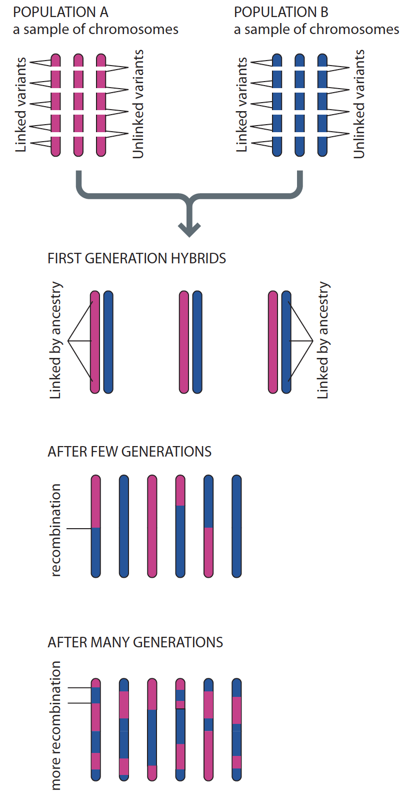Fig. 1: Admixture generates LD between loci. Figure from Human Evolutionary Genetics (2nd Ed).

Problem is, we can’t know the ancestry at a locus. Chromosomes are not painted red or blue (or which population they come from). What we can find out are the genotypes (by genotyping/sequencing). Does admixture induce correlations between genotypes at unlinked loci? Yes, but this correlation depends on a number of things and to develop a more nuanced (and quantitative) understanding, we need to do some math.

Factors affecting admixture LD

Let there be two (randomly mating) populations that have been reproductively isolated for enough time for there to be systematic frequency differences between them. Denote \(X_1^A\) and \(X_2^A\) as the genotypes at locus A for an individual sampled randomly from population 1 and 2, respectively, such that \(\mathbb{E}(X_1^A) = f_1^A\) and \(\mathbb{E}(X_2^A) = f_2^A\) where \(f_1^A\) and \(f_2^A\) are the frequencies of the \(A\) allele in population 1 and 2, respectively. Similarly, denote the genotype and frequency of another (unlinked) locus \(B\) on a different chromosome as \(X_1^B\) and \(f_1^B\), respectively.

Statistically speaking, LD is a measure of the covariance in genotypes between two loci. For population 1, the covariance, \(D = cov(X_1^A, X_1^B) = \mathbb{E}(X_1^{AB}) - \mathbb{E}(X_1^A)\mathbb{E}(X_1^B)\) ². Here, \(\mathbb{E}(X_1^{AB})\) is the expectation of observing alleles \(A\) and \(B\) together, which is equal to the frequency of the \(AB\) haplotype denoted by \(f_1^{AB}\). In a randomly mating population, the frequency of the haplotype is equal to the product of the frequency of the individual loci, \(f_1^{AB} = f_1^A f_1^B\) and \(D = f_1^{AB} - f_1^Af_1^B = 0\).

Now, imagine that there is an admixture event where individuals from populations 1 and 2 are put together in a single population in proportions of \(\alpha\) and \(1-\alpha\), respectively. In this meta-population, the expected frequencies of the \(A\) and \(B\) alleles are \(\alpha f_1^A + (1-\alpha)f_2^A\) and \(\alpha f_1^B + (1-\alpha)f_2^B\), respectively ³. Similarly, the expected frequency of the \(f^{AB}\) haplotype is \(\alpha f_1^{AB} + (1-\alpha)f_2^{AB}\). The LD between the two loci in the admixed population is therefore:

\[\begin{aligned} D & = f^{AB} - f^Af^B \\ & = \{\alpha f_1^{AB} + (1-\alpha)f_2^{AB}\} - \{\alpha f_1^A + (1-\alpha)f_2^A\}\{\alpha f_1^B + (1-\alpha)f_2^B\}\\ & = \{\alpha f_1^{AB} + (1-\alpha)f_2^{AB}\} - \{\alpha^2 f_1^Af_1^B + \alpha(1-\alpha)f_1^Af_2^B + \alpha(1-\alpha)f_2^Af_1^B + (1-\alpha)^2 f_2^Af_2^B \} \\ & = \alpha f_1^Af_1^B + \alpha^2 f_1^Af_1^B + (1-\alpha)f_2^Af_2^B - (1-\alpha)^2f_2^Af_2^B - \alpha (1-\alpha)f_1^Af_2^B - \alpha (1-\alpha)f_2^Af_1^B \\ & = \alpha(1-\alpha)f_1^Af_1^B - \alpha(1-\alpha)f_1^Af_2^B + \alpha(1-\alpha)f_2^Af_2^B - f_1^Af_2^B\alpha(1-\alpha) \\ & = \alpha(1 - \alpha)\{ f_1^Af_1^B - f_1^Af_2^B + f_2^Af_2^B - f_2^Af_1^B\} \\ & = \alpha(1-\alpha)\{ f_1^A(f_1^B - f_2^B) - f_2^A(f_1^B - f_2^B) \} \\ & = \alpha(1-\alpha)\{ (f_1^A - f_2^A)(f_1^B - f_2^B)\} \end{aligned}\]

This shows that the admixture LD between the genotypes at two loci depends on two things: (i) the product of the allele frequency difference between the two populations \((f_1^A - f_2^A)(f_1^B - f_2^B)\) ⁴ and (ii) the admixture fraction \(\alpha\). Let’s get an intuitive understanding of the relationship between admixture LD and these two quantities with a plot.

#create matrix to store D
dmat = matrix(NA, nrow = 11, ncol = 11)
alpha = seq(0, 1, 0.1) # range of values of admixture fraction
fdiff = seq(0, 1, 0.1) # range of values of frequency difference at locus A. assume difference at locus B is 1.

for(i in 1:11){
  for(j in 1:11){
    dmat[i,j] = alpha[i]*(1 - alpha[i]) * 1 * fdiff[j]
  }
}

image(dmat, main = "Admixture LD", col = heat.colors(12), 
      xlab = bquote("Admixture fraction"~alpha), ylab = "Frequency difference at locus B")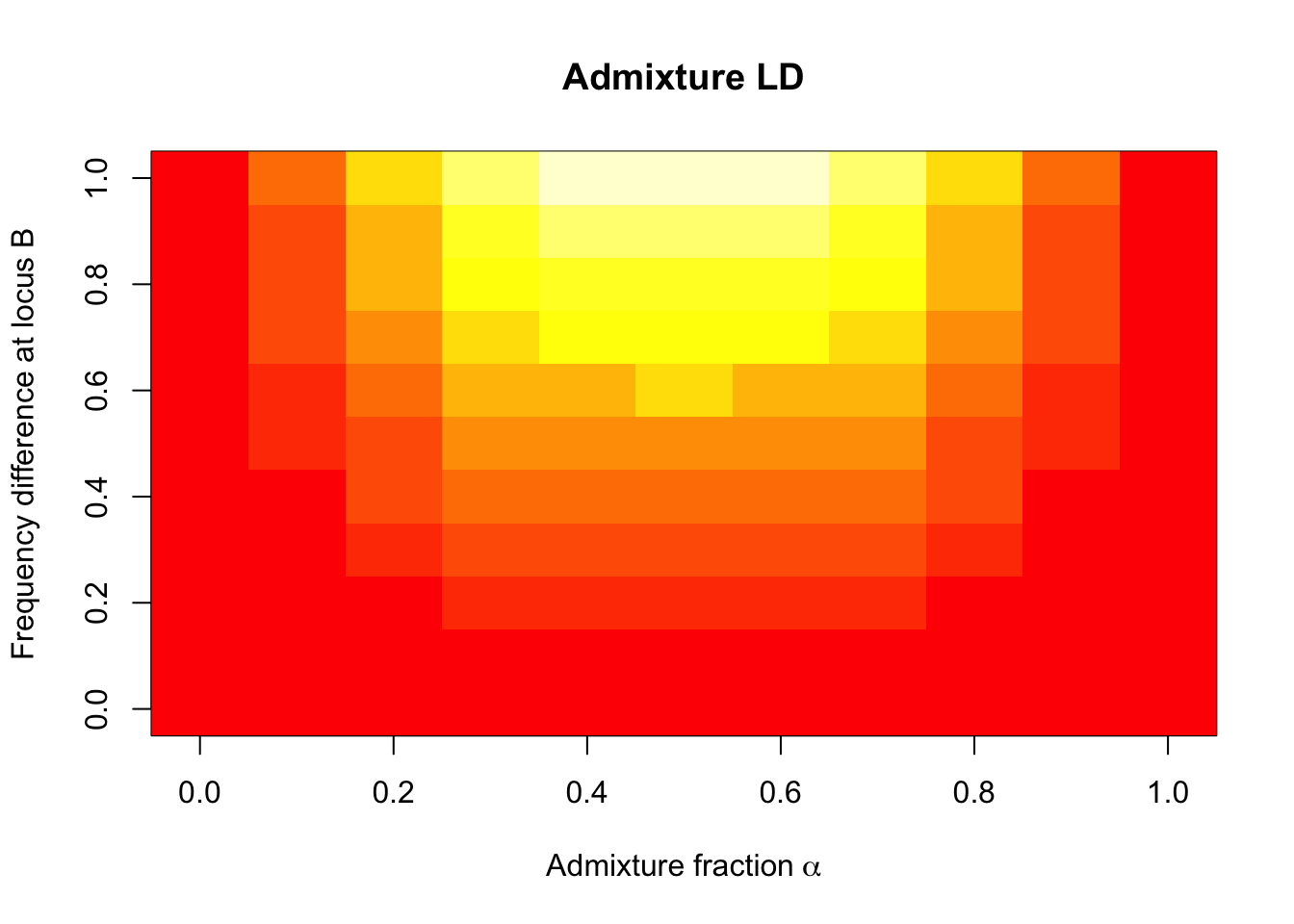

We can tell that there will be no LD between unlinked loci (i.e. \(D = 0\) where tiles are red) in an unadmixed (randomly mating) population (i.e. when \(\alpha = 0\) or \(\alpha = 1\)). \(D = 0\) also when the allele frequency at either of the two loci are equal between the two populations (i.e. \(f_1^A - f_2^A = 0\) or \(f_1^B - f_2^B = 0\)). For any other situation (\(\alpha >0\) & \(|f_1^A - f_2^A| > 0\) & \(|f_1^B - f_2^B| > 0\)), unlinked loci will be correlated across the genome (\(D > 0\) where tiles are more yellow). The requirement that \(|f_1^A - f_2^A|\) and \(|f_1^A - f_2^A|\) be greater than 0 means that admixture LD only affects loci where the frequencies are different between the two populations, the admixture LD increasing with the difference in frequency.

Admixture LD is maximized (bright yellow region) when two conditions are met: (i) when \(\alpha = 0.5\) (i.e. each population contributes to the admixture event equally), which would make \(\alpha(1-\alpha) = 0.25\), and (ii) when the product of allele frequency difference \((f_1^A - f_2^A)(f_1^B - f_2^B)\) is 1. The latter is only possible if both \(f_1^A - f_2^A = f_1^B - f_2^B = 1\), i.e. if one allele is fixed in one population and absent in the other population.

Admixture LD decays pretty rapidly with random mating

So far we’ve only considered LD right after admixture. Admixture LD between unlinked loci decays pretty rapidly after admixture in a randomly mating population due to recombination between loci and independent assortment (see Fig. 1 again). Let’s denote admixture LD in generation \(t\) since admixture as \(D^t\). In a randomly mating population arising from a single admixture event, \(D^t = D^0 (1 - r)^t\) ⁵ where \(D^0\) is the admixture LD observed at the time of admixture and \(r\) is the recombination fraction between the two loci. Let’s plot the decay of admixture LD as a function of the \(r\) assuming the maximum possible value \(D^0\) can take (i.e. 0.25).

suppressPackageStartupMessages(library(ggplot2))

#range of values of r (recombination fraction)
r = seq(0, 0.5, 0.1)
dtmat = matrix(NA, nrow = 6, ncol = 10) # matrix to store values of dt

#max possible value of D0 is when alpha = 0.5 and when freq diff is 1. 
#this leads to a max value of 0.25 

for(i in 1:6){
  dt = 0.25
  for(j in 1:10){
    dtmat[i,j] = dt
    dt = dt*(1 -r[i])^j
  }
}

dtmat = reshape2::melt(dtmat)

colnames(dtmat) = c("r","g","Dt")
dtmat$r = (dtmat$r - 1)/10

ggplot(dtmat, 
       aes(g, Dt, group = r, 
           color = as.factor(r)))+
  geom_line()+
  theme_classic()+
  theme(axis.text = element_text(size = 14),
        axis.title = element_text(size = 16),
        legend.title = element_text(size = 14))+
  scale_color_viridis_d()+
  scale_x_continuous(breaks = c(1:10))+
  labs(x = "Generations since admixture (t)",
       y = bquote(D[t]),
       color = "r")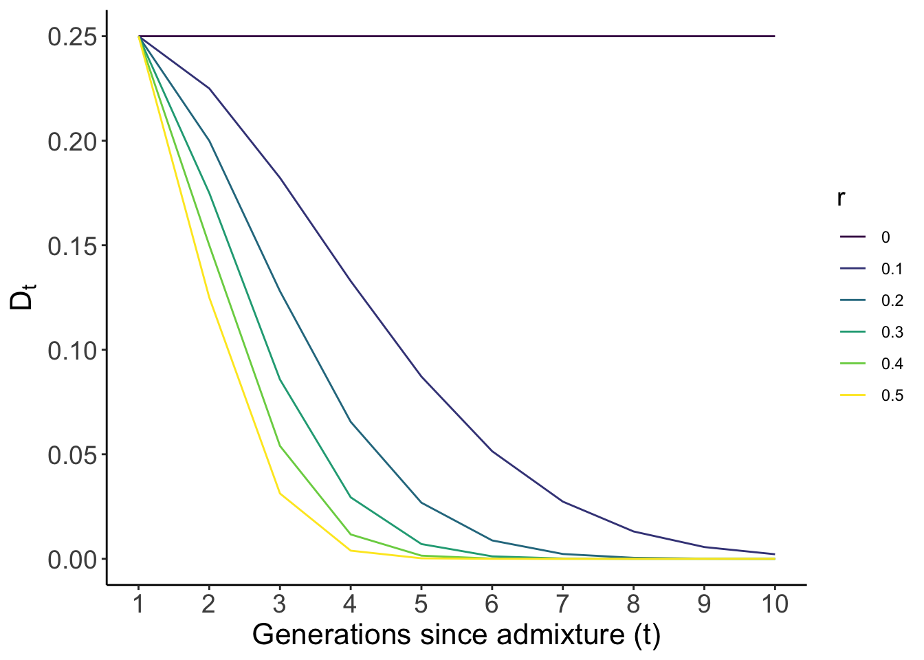

As you can see, \(D\) decays very quickly between loci, but especially when the loci are not unlinked (i.e. \(r = 0.5\), yellow line), reaching almost neglegible values just after 4 generations of random mating. However, the rate of decay shown here is if the admixed population were mating randomly. Admixture LD will decay more slowly in a population with ancestry-based assortative mating (i.e. where individuals prefer to mate with others of similar ancestry) and/or if the admixture is continuous (i.e. with an continuous influx of individuals from one or both of the ancestral populations) as opposed to occurring in a single event. Why that happens is beyond the scope of this post but you should look up Pfaff et al. 2001 and Zaitlen et al. 2017 for a deeper treatment (with nice and clear notation) of this topic.

LD between unlinked loci can also be generated due to population structure or assortative mating in the population (non-random mating broadly). Thus, admixture LD is a special instance of a more general phenomenon whereby demographic processes (e.g. population structure and assortative mating) can induce correlations across the genome. The correlations between unlinked loci that arise due to population structure and admixture is sometimes called the multi-locus Wahlund effect. Sometimes people call this type of LD gametic phase disequilibrium (how’s that for a mouthful) to distinguish it from LD due to physical linkage.